Haskell for numerical computation?

software

programming

Published

September 5, 2023

Why Haskell?

Recently, I have been experimenting with Haskell which I find to be quite enjoyable to program in, thanks to its unique programming paradigm. So much so that I am considering using it for numerical computations in my research.

Side-effects refers to having an effect on the “outside world” such as printing a string to terminal or writing to a file etc. Of course, we do want some side-effects for the program to do anything useful. In Haskell, side-effects are handled by monads, which is a beast of a topic on its own. Monads allow the pure and impure (side-effects) to be clearly separated in Haskell.

Haskell (named after logician Haskell Curry) is a purely functional programming language in the mathematical sense. Every function in Haskell simply takes an input and returns an output—nothing more, nothing less. It cannot mutate variables, and it cannot produce side-effects.

Purely functional programming languages are typically declarative, i.e., one does not write step-by-step instructions like imperative languages such as Python, C, C++, etc. For example, there are no loops in Haskell; one has to rely on recursion or functions such as ‘fold’ and ‘scan’.

The two main reasons for my consideration to use it for numerical computations are:

Conciseness: Haskell’s declarative style greatly increase its conciseness. Prototyping and experimentation are frequent in computational research. Concise codes can reduce this programming time, and allow faster prototyping.
Safety and correctness: A small bug in numerical computational would not raise any error. Instead, it manifests in computed results or plots, masquerading as valid or even novel results. If these bugs are not identified, one might publish a paper with faux results.
- Haskell’s static typing can serve as an additional check to reduce bugs.
- Its declarative approach means that codes are written in easily verifiable expressions, like in mathematics, rather than imperative statements that are often prone to bugs or human error.
- Immutability and the absence of side-effects in functions can also reduce hidden bugs. For instance, the risk of a function modifying a variable without the coder’s knowledge is mitigated, and parallel computations are less likely to produce incorrect results due to variable mutations in multiple threads.

I am neither a software developer nor am I computer science trained, and so some technical aspects of the language might escape me. Therefore, in this article, we will only examine some simple examples to compare traditional imperative languages like Python with purely functional Haskell.

Some examples

Sum: recursion

Ignoring the fact that the function sum is built-in in both Python and Haskell, let’s see how one might write a sum function that sum all the elements in a list.

Python
Haskell

def sum(xs):
    sum_all = 0
    for x in xs:
        sum_all += x
    return sum_all

sum :: [Float] -> Float
sum [] = 0
sum (x:xs) = x + sum xs

In the imperative Python example, we tell the program what to do step-by-step: first initialize an accumulator sum_all to 0, then loop through each elements in the list and add them to the accumulator.

One might notice that functions are applied without parenthesis, i.e., applying a function foo on a variable x, is typically foo(x), but would be foo x in Haskell. The reason for this has something to do with the concept of “currying” which we will see later.

On the other hand, in the declarative Haskell example, we state that the sum of a list is simply the first element x plus the sum of the rest of the elements xs. This will then carry on recursively. As with all recursive functions, we require a base case to end the recursion, which is specified by sum [] = 0, which states to return 0 if the input to sum is an empty list. This ability to define the sum function twice with sum [] = 0 and sum (x:xs) = x + sum xs, is simply pattern matching.

Finally, Haskell is statically typed, i.e., the types of the inputs and outputs of the function can be specified which in our case is sum :: [Float] -> Float, which states that the function sum takes in a list of floats [Float] and returns a single float Float. This type declaration looks similar to how one might write f: X \to Y mathematically for a function y = f(x), where x \in X, and y\in Y.

Tensor product: reduction and accumulation

Here is a common example in quantum information/computation, where we have some quantum states that are complex matrices, and we want to perform a tensor product on them so that we can operate on them collectively.

Given a list of matrices, the function tensor_all returns the tensor product of all the elements of the list in sequence, e.g., given the list of matrices Ms = [A, B, C], tensor_all(Ms) should return their tensor product A\otimes B\otimes C.

Python
Haskell

import numpy as np

def tensor_all(Ms):
    tensor_prod = 1
    for M in Ms:
        tensor_prod = np.kron(tensor_prod, M)

    return tensor_prod

import Numeric.LinearAlgebra

tensor_all :: [Matrix C] -> Matrix C
tensor_all = foldl kronecker 1

Imperatively in the Python example, we loop through each element of the list and apply the tensor product (kronecker product np.kron) element-by-element with an accumulator, i.e., in the first loop we have (1) \otimes A, in the second loop we have (1\otimes A) \otimes B, in the third loop we have (1\otimes A \otimes B) \otimes C, and so on and so forth, where our accumulator tensor_prod is the value in the parenthesis, is initialized as 1, and is updated every loop.

Note we have used the hmatrix library which is imported by import Numeric.LinearAlgebra. This documentation is a good resource for a comparison between hmatrix and Python’s numpy.

In Haskell, it should be obvious that we can perform a recursion like the case for sum. However, here we introduced the function foldl, which stands for “fold left”. foldl takes in a binary function (in this case kronecker), the initial accumulator (in this case 1), and a list (e.g., [a, b, c]). It then returns kronecker(kronecker(kronecker(1, a), b), c). There is also foldr, or “fold right”, which instead returns kronecker(a, kronecker(b, kronecker(c, 1))).

Point-free style programming

Note that in the Haskell example, we could have written the function as tensor_all ms = foldl kronecker 1 ms, where the input to the function, the list of matrices ms, is specified. However, since ms is simply the input to the corresponding functions on both sides of the expression, we can omit it and simply write tensor_all = foldl kronecker 1. This is referred to as point-free style programming.

If instead, we want to “accumulate” the result of each loop into a list, i.e., we want the function to return [A, A \otimes B, A\otimes B\otimes C], then, in the Python example we have to append the accumulator tensor_prod in each loop into a list. On the other hand, in the Haskell example, we can simply replace foldl with scanl.

Python
Haskell

import numpy as np

def tensor_all(Ms):
    tensor_prod = 1
    tensor_prod_list = []
    for M in Ms:
        tensor_prod = np.kron(tensor_prod, M)
        tensor_prod_list.append(tensor_prod)

    return tensor_prod_list

import Numeric.LinearAlgebra

tensor_all :: [Matrix C] -> [Matrix C]
tensor_all = scanl kronecker 1

Folds and scans are part and parcel of a functional programmer, and are common in functional programming languages, as well as array programming languages. Typically, they are referred to as reduction and accumulation, e.g., in the array programming languages NumPy, Julia, and R, folds and scans are called reduce and accumulate.

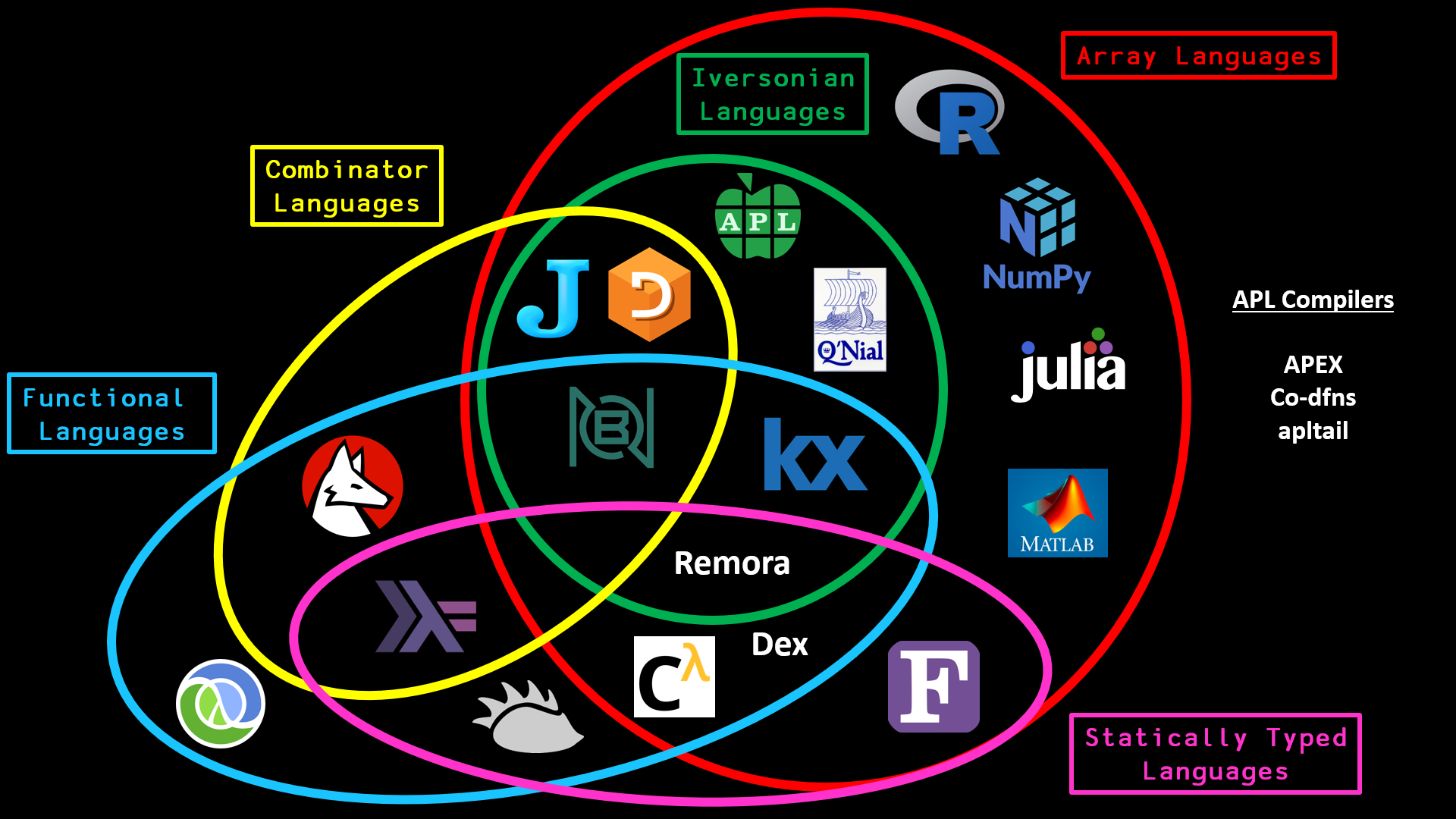
If you would like to know more about array languages, and how they compare to functional languages like Haskell, I highly recommend the youtube channel code_report.

Collision model: currying and laziness

Let’s consider a less simple example to reveal more of Haskell’s features:

A superconducting qubit \rho (rho) is sensitive to heat, and is continuously undergoing a thermalization process. We can model this thermalization process with a collision model, where the qubit evolves via repeated “collision” with different qubits at each discrete time step for n (n) number of time steps. The collision is implemented by the function collision. We want to determine how the von Neumann entropy of \rho, S(\rho), changes in each collision up till n time steps. The calculation of the von Neumann entropy is implemented by the function entropy.

For completeness, the function collision performs the operation of \rho_{t+1} = \sum_i K_i \rho_t K_i^\dagger, where K_i are Kraus operators, and the function entropy computes S\left(\rho_t\right) = -\mathrm{Tr} \left(\rho_t \log \rho_t\right). Therefore, what we want is simply the list of \small[S(\rho_0), S(\rho_1), \ldots, S(\rho_{n-1})]

This might look complicated if one does not know quantum mechanics. However, if we assume that the collision and entropy calculations are done for us in the functions collision and entropy, then we simply want a list of n entropy values, i.e., entropy_list = [entropy(rho), entropy(collision(rho)), entropy(collision(collision(rho))),...].

Python
Haskell

import scipy as sp

def collision(ks, rho):
    return sum([k @ rho @ k.conj().T for k in ks])

def entropy(rho):
    return - np.trace(rho @ sp.linalg.logm(rho))

def calc_entropies(ks, rho, n):
    entropy_list = []
    for _ in range(n):
        rho_entropy = entropy(rho)
        entropy_list.append(rho_entropy)
        rho = collision(ks, rho)

    return entropy_list

collision :: [Matrix C] -> Matrix C -> Matrix C
collision ks rho = sum [k <> rho <> tr k | k <- ks]

entropy :: Matrix C -> Float
entropy rho = - trace (rho <> logm rho)
  where
    logm = matFunc log

calc_entropies :: [Matrix C] -> Matrix C -> Int -> [Float]
calc_entropies ks rho n = map entropy rho_list
  where
    rho_list = take n (iterate (collision ks) rho)

Extra things to note for the Haskell example

Similar to Python, Haskell has list comprehension, which has a mathematical syntax as seen in the function collision, e.g.,
```
example = [p * q | p <- ps, q <- qs, p >= 5, q /= 0]
```
would give a list of the set \{pq\ |\ p \in P,\ q \in Q,\ p \geq 5,\ q \neq 0 \}.

On the other hand, Python’s list comprehension is less concise:
```
example = [p * q for p in ps for q in qs if p >= 5 and q != 0]
```

In the entropy and calc_entropies functions, we have used the where keyword, which allows us to break a function into smaller constituents, e.g.,

exampleFunc a b c = n / d
  where
    n = x + y
    d = x - y
    x = a + b + c
    y = a * b * c

Alternatively, we can also use the let and in keyword:

exampleFunc a b c =
  let
    n = x + y
    d = x - y
    x = a + b + c
    y = a * b * c
  in
    n / d

The Python example, being imperative, should be self-explanatory. Instead, we are interested in the Haskell example, specifically the calc_entropies function, which might look arcane if one does not know common functional programming functions such as map, take, and iterate. Let’s look at this line-by-line.

Currying

The very first line of the calc_entropies function is the type signature of:

\mathtt{calc\_entropies :: [Matrix\ C]\ -> Matrix\ C\ -> Int\ -> [Float]}

which states that the function calc_entropies takes in a list of complex matrix, a complex matrix, and an integer, and returns a list of floats. The list of complex matrix refers to the Kraus operators K_i used in the collision function, the complex matrix refers to rho or \rho, the integer refers to n, while the list of floats refers to the output entropy_list.

One might notice that [Matrix C] -> Matrix C -> Int -> [Float] doesn’t seem to make a clear distinction between inputs and outputs. This has to do with the concept of partial function application, or currying (also named after Haskell Curry).

Implicitly, what’s happening is the following:

\mathtt{calc\_entropies :: [Matrix\ C]\ ->\ } \underbrace{\mathtt{Matrix\ C\ -> Int\ -> [Float]}}_\text{function $f$} f\ \mathtt{:: Matrix\ C\ ->\ } \underbrace{\mathtt{Int\ -> [Float]}}_\text{function $g$} g\ \mathtt{:: Int\ -> [Float]}

where the function calc_entropies takes in [Matrix C] as its input, and returns a function f as its output. The function f then takes in Matrix C as the input and returns another function g as the output. Finally, the function g takes in Int as the input and returns [Float] as the final output. This means that functions in Haskell are indeed pure in that they only take in one input and one output, and any functions that appear to take in multiple inputs are in fact taking in only one input and returning a function that takes in also one input, and so on and so forth. This is called currying. Because of this, we can also apply the functions “partially”, for example:

f a b = a + b
g = f 5

where we only provide one argument to f when it is expecting two, to create a new function g. This means that f 5 10 and g 10 would give the same output of 15. Currying or partial function application can be a powerful tool for the abstraction and expressiveness of your code.

Example of the usefulness of currying

Unitary operations are common in quantum mechanics, and are how quantum computers perform computations on quantum states or qubits. They are defined as follows: |\psi'\rangle = U |\psi\rangle.

We can define a function unitary_oper to implement this.

Python
Haskell

def unitary_oper(U, ket):
    return U @ ket

unitary_oper :: Matrix C -> Matrix C -> Matrix C
unitary_oper u ket = u <> ket

There are many common unitaries U used in quantum computations, referred to as quantum logic gates. For example there are the Pauli X gate and the Hadamard gate which are defined as X = \begin{pmatrix} 0 & 1 \\ 1 & 0 \end{pmatrix},\quad H = \frac{1}{\sqrt{2}} \begin{pmatrix} 1 & 1 \\ 1 & -1 \end{pmatrix}.

Currying or partial-function application allows us to easily define these new gate operations on top of the existing unitary_oper function:

pauli_x = unitary_oper (2><2) [0, 1, 0, 1]
hadamard = unitary_oper (cmap (/ sqrt 2) (2><2) [1, 1, 1, -1])

We can then easily apply the Pauli X and Hadamard gates on a qubit |0\rangle = [1, 0]^T with pauli_x (2><1) [1, 0] and hadamard (2><1) [1, 0]. This can make the code more concise and clearer.

Lazy evaluation

Moving on to the function itself:

calc_entropies ks rho n = map entropy rho_list
  where
    rho_list = take n (iterate (collision ks) rho)

The first line features the function map, which is another part and parcel of the functional programmer. It simply apply a function to every element of a list:

\underbrace{\mathtt{map\quad entropy}}_\text{apply entropy function to each element of}\quad \mathtt{rho\_list}

and has the corresponding Python code of

entropy_list = [entropy(rho) for rho in rho_list]

# or alternatively
entropy_list = []
for rho in rho_list:
    entropy_list.append(entropy(rho))

Finally, in the last line we have

\mathtt{where\quad rho\_list} = \underbrace{\mathtt{take\quad n}}_\text{take first $n$ of}\quad \underbrace{\mathtt{(iterate\quad (collision\quad ks)\quad rho)}}_\text{returns an infinite-sized list of [rho, collision(rho), collision(collision(rho)),...]} which gives rho_list = [rho, collision(rho), collision(collison(rho)),...] up till n number of elements in the list.

Also note that we can reduce the number of parenthesis by using $ instead, e.g., rho_list = take n $ iterate (collision ks) rho.

It might be quite surprising that the iterate function returns an infinite-sized list. For example, iterate add1 10 gives [11, 12, 13, 14, 15, ...] to infinity, where the function add1 is applied on 10 ad infinitum. If we were to write the corresponding Python code for rho_list = take n (iterate (collision ks) rho), it might look something like

rhos = []
while True:
    rhos.append(rho)
    rho = collision(ks, rho)

rho_list = rhos[:n]

which runs forever and result in a list of infinite size. However, this is not a problem in Haskell, thanks to the fact that Haskell is lazy-evaluated. This means that Haskell only evaluate values when required, and so since we only require the first n elements of the infinite list, Haskell only evaluate that first n elements.

If this Python code is lazy-evaluated like in Haskell, one might imagine that the program looks ahead and saw that it only require the first n elements as stated in rho_list = rhos[:n], and so it stops the while True loop after only running n times.